Generative surrogate modelling for the efficient design optimization of an RF component

Abstract

Accurate and efficient design of millimeter-wave components is critical for sixth-generation (6 G) wireless systems, particularly at the D-band where low-loss interconnects are required. Vertically aligned carbon-nanotube (VACNT)–based air-filled waveguides (AFWGs) have recently been introduced as a promising alternative to conventional metallic structures, offering reduced propagation losses and wafer-level compatibility. However, their optimization remains dependent on full-wave solvers such as HFSS, where large parametric sweeps are computationally prohibitive. This work introduces a rank-reduction autoencoder (RRAE) as a machine-learning-based surrogate modeling technique incorporating a truncated principal component analysis (PCA) stage enabling robust performances, reliable interpolation and constraint-preserving sampling based on small datasets. Trained on 421 HFSS simulations only, the RRAE managed the retrieval of 5 unique optimized VACNT-AFWG designs with operational bandwidths between 135 and 155 GHz. It has been benchmarked against a direct encoder–decoder regression baseline sharing the same backbone but without the rank-reduction stage that did not produce any HFSS-confirmed valid design in the proposed screening workflow. The RRAE hence presents itself as a scalable solution for surrogate-assisted optimization and shows to be a promising candidate for the design of next-generation low-loss waveguide technologies.

Introduction

The Sixth-generation (6 G) wireless communication technology aims to provide ultra-high data rates (up to 1 Tbps), negligible latency, energy efficiency, global coverage, and intelligent connectivity on a global scale [1]. Millimeter-wave frequencies, especially the D-band, are considered ideal for such applications. As in other frequencies, D-band on-chip transceivers will be integrated on PCBs and up-conversion mixers relying on hollow metallic waveguides (WGs), necessitating efficient WG–PCB transitions. This improved the performance of CMOS active components at mm-wave frequencies. These requirements highlight the need for compact, high-performance passive devices. At D-band and beyond, traditional planar transmission lines such as microstrip or CPW suffer from pronounced dielectric and radiation losses, as well as strong electromagnetic coupling between adjacent conductors, which collectively degrade signal integrity and system performance [2]. Conventional volumetric fabrication techniques also add cost and complexity. A new class of cost-effective, high-efficiency, integrated passive devices is needed. Air-filled waveguides (AFWGs) provide a promising low-loss alternative, but standard metallic implementations are still bulky and expensive, limiting their use in compact packaging. Recently, vertically aligned carbon-nanotube (VACNT)–based AFWGs have been introduced as a novel solution, combining low-loss propagation with compatibility for wafer-level integration [3, 4]. Section “Optimization of a vacnt-based air-filled waveguide for millimeter wave” will be dedicated to the optimization of such AFWG structure for D-band applications.

In this context and to answer the time, cost and accuracy constraints of industrial design workflows, recent research has focused on electromagnetic design optimization for RF applications [5]. Researchers have proposed machine learning (ML) tools for waveguide, filter, and microwave component optimization [6,7,8,9,10]. These studies show that ML and inverse-design processes accelerate product development. Parametric models directly map input parameters (e.g., material or geometric properties) to system outputs, enabling real-time predictions and advanced applications like inverse identification, real-time control, and optimization [11,12,13].

The authors in [14] for instance use convolutional neural networks trained on 400,000 simulations for the inverse design of complex multi-ports circuits restricted to grid-like representations to fit their chosen model architecture. Alternatively, in [15] the authors propose another two-step deep learning method to optimize the design of patch antenna arrays based on 70,000 sets of radiation patterns issued from 5 preset designs to limit the number of optimization variables. Although successful in improving optimality, these examples highlight two common challenges of AI-based optimization: data consumption and design space representation.

These challenges are closely linked. Large datasets are often required when the model must learn both the electromagnetic response and the structure of the admissible design space from examples alone. Conversely, reducing the design space to a small set of predefined parameters can make the learning problem easier, but may limit the flexibility of the optimization process and requires the designer to explicitly manage parameter correlations and feasibility constraints. In RF component design, where each data point may require a costly full-wave simulation, an effective surrogate framework should therefore not only predict responses accurately, but also provide a representation of the design space that can be efficiently explored.

Effective optimization necessitates a comprehensive exploration of the design space, which in turn requires a rigorous and well-defined representation.

For this purpose, AI models must be trained on sufficiently rich datasets to ensure adequate generalization to unseen designs. At the same time, the cost of acquiring such datasets must remain compatible with the constraints of an optimization framework, hence motivating the development of data-efficient methodologies.

Equally as important is the representation of the design space itself, as it governs the efficiency of the exploration process. Although parameterization offers a natural means of representation, it quickly becomes challenging or inefficient in the presence of strong parameter correlations or in non-parametric settings such as for the representation of complex shapes or topologies for instance.

Mitigating these issues is an active research topic. On the one hand, several methods have been developed [16, 17] to increase the reliability of surrogate models trained on small datasets. Among them common solutions are physics informed neural networks (PINN) or transfer and meta learning strategies, leveraging pre-existing knowledge to guide learning efficiently. While effective in alleviating data scarcity, these methods inherently depend on the availability and suitability of such prior knowledge, which may not always be guaranteed.

On the other hand, tools are also developed in order to improve data exploration, particularly in inverse and generative electromagnetic design workflows [18]. A widely adopted strategy is the integration of Variational AutoEncoders (VAE) and Generative Adversarial Networks (GAN) into a single VAE-GAN framework [19, 20]. The VAE constrain the latent data representations to follow a specific statistical distribution therefore allowing sampling from it while the GAN ensures the generation of high quality samples. This type of approach however often requires substantial amount of data to be trained and lacks control and interpretability when it comes to generation.

Combining both methodologies to address simultaneously frugality and explorability however remains a significant challenge, largely due to their inherently conflicting requirements.

With the advent of future RF modules and systems, the accurate design of components, typically relying on full-wave electromagnetic solvers such as HFSS [21], is becoming increasingly challenging and time-consuming [22]. The large parametric sweeps and optimization loops involved, render brute-force optimization inefficient even with current machine learning frameworks. Bridging both frugal and explorable methodologies will therefore become essential to enable the development of next generations of RF components and systems in a time and cost efficient manner.

To this end, we introduce in this work a rank-reduction autoencoder (RRAE) framework as a frugal yet generative surrogate modeling approach for RF and microwave devices. By embedding a truncated principal component analysis (PCA) stage into the latent space of an autoencoder, we enforce a low-rank structured parametrization of the latent space, enabling robust interpolation and constraint-preserving generative sampling. This architecture combines regression-based surrogates and generative models while mitigating their respective weaknesses. To demonstrate its potential, we apply the method to the design optimization of a VACNT-based AFWG targeting the D-band, using a modest dataset of 421 HFSS simulations. The method is evaluated against a controlled direct encoder-decoder regression baseline sharing the same backbone but without the rank-reduction stage. This comparison separates full-band reconstruction fidelity from design-space exploration capability: both models are assessed as response predictors, while the added value of the RRAE lies in its ability to generate and screen candidate designs within the learned low-rank manifold. The proposed framework achieves sub-dB median error in return-loss prediction, reduces evaluation time from minutes to milliseconds, and identifies multiple new valid designs satisfying the D-band requirements.

In this paper, Sect. “Generative surrogate modeling” is dedicated to the introduction of the RRAE framework and its potential in engineering optimization. A use-case application is detailed in Sects. “Optimization of a vacnt-based air-filled waveguide for millimeter wave” and  “Results and discussion” is focused on highlighting and discussing the results.

Generative surrogate modeling

To address the computational challenges of high-fidelity simulations in optimization, we explore surrogate modeling approaches that enable efficient exploration of the design space defined by a number of parameters grouped in a vector $\mathbf {\mu }$.

First, a Design of Experiments (DoE) is defined, consisting of D parameter choices: $\mathbf {\mu }^1,..., \mathbf {\mu }^D$. Now, for each parameters choice, a high fidelity simulation is performed, that results in the solutions $\textbf{X}^1,..., \textbf{X}^D$, each expressed, without loss of generality as a vector.

The surrogate consists of a regression that associates to any parameters choice $\mathbf {\mu }$ the associated solution $\textbf{X}$. The regression can be expressed as $\textbf{X}(\mathbf {\mu })$.

This functional expression can be constructed following different strategies, all of them exploiting the reproduction property, that is, $\tilde{\textbf{X}}^i \equiv \textbf{X}(\mathbf {\mu }^i) \approx \textbf{X}^i$, $i=1,..., D$.

Reduction

As the size of the data $\textbf{X}$ is substantial in general, its reduction facilitates the regression construction. For that reason data reduction is usually employed.

That reduction can be:

• Linear, for example by performing the singular value decomposition (SVD) of the so-called snapshots matrix $\mathbb {X} = [\textbf{X}^1 \cdots \textbf{X}^D]$. A reduced basis $\{ \textbf{U}^1,...,\textbf{U}^R\}$ can then be obtained from the truncated SVD of matrix $\mathbb {X}$, where the retained modes (and its number) ensures approximating the data $\textbf{X}^i$, $\forall i$, up to a selected degree of precision. Thus, $\textbf{X}$ is expected being expressed from:

  $$\begin{aligned} \textbf{X}= \sum \limits _{i=1}^R c_i \textbf{U}^i, \end{aligned}$$

  (1)

  that reduces to R scalar regressions $c_i$, $\forall i$ [23].

• Nonlinear reduction, by making use for example of an autoencoder [24,25,26]. The latter maps data $\textbf{X}$ into $\textbf{Y}$, $\textbf{Y}(\textbf{X})$, defined in a space with the smallest dimensionality R, enabling to recover the initial data from an inverse mapping. If the direct mapping (the so-called encoding) is performed by a neural network involving the parameters $\mathbf {\theta }^e$, $\textbf{Y}= \mathcal {N}_{\mathbf {\theta }^e}(\textbf{X})$, and the inverse one (the decoder) is ensured by the associated decoder neural network $\tilde{\textbf{X}}=\mathcal {N}_{\mathbf {\theta }^d}(\textbf{Y})$, $\mathbf {\theta }^d$ being the associated decoder parameters, both network parameters $\mathbf {\theta }^e$ and $\mathbf {\theta }^d$ should be computed from the available data, during the so-called model training. Thus, from the available data $\textbf{X}^i$, $i=1,..., D$ the reproduction condition reads, $\forall i$, $\tilde{\textbf{X}}^i \approx \textbf{X}^i$, with $\tilde{\textbf{X}}^i = \mathcal {N}_{\mathbf {\theta }^d}(\mathcal {N}_{\mathbf {\theta }^e}(\textbf{X}^i))$.

Exploration

The linear reduction method guarantees the mathematically optimal linear projection minimizing reconstruction error. In addition, it is computationally efficient and interpretable. However, it is unable to handle nonlinear correlations and thus its application becomes limited for complex data and in nonparametric settings. The use of nonlinear methods such as autoencoders solves this issue but do not ensure optimality and therefore can lead to inaccuracies when it comes to generation.

To illustrate this limit, let us consider M-pixels images representing circles of fixed diameters only allowed to move along the diagonal of the image as pictured in Fig. 1a

Now, if the data representing each image $\textbf{X}^i$, $i=1,..., D$ is used to train an autoencoder (as discussed above), the autoencoder will find (if the amount of data is enough) that the data $\textbf{X}^i \in \mathbb {R}^M$, $\forall i$, can be mapped into a one-dimensional space, $Y^i \in \mathbb {R}$, $\forall i$. By considering other values of Y, $Y \ne Y^i$, $\forall i$, one could imagine that circles in as many positions as possible could be generated by sampling this reduced space. However this is not always correct and the latent space in which Y is defined fails in many cases to enable robust generation or interpolation, especially in spaces of higher dimension. We illustrate this drawback in Fig. 1bwhere a new position is sought by interpolating (linearly) between the two neighbors (top-left and bottom-right). Due to inaccuracies in defining the latent space with the autoencoder, the resulting data-point leaves the one-dimensional manifold and the image produced by the decoder will differ from the expected circle.

Fig. 1

a Pixel-based images of fixed-radius circles moving along the diagonal; b Example of interpolation outside the latent manifold

As introduced previously, variational autoencoders successfully fix this issue by enforcing the learned latent space to follow a set statistical distribution, but they are much more expensive to train. Moreover, performances are usually hindered by this harsh constraint and must usually be combined with generative adversarial networks, whose discriminators enhance the quality of generated data [19].

In our recent works [27] we followed a different route for ensuring robust generation and interpolation by combining both reduction approaches to benefit from both their advantages and mitigate their limits. We enforce that the latent space becomes a linear vector space. This task can be performed by adding a truncated PCA (principal component analysis) between the encoder and the decoder that is expected to provide a reduced number of orthonormal modes $\{ \textbf{U}_1, \textbf{U}_2,..., \textbf{U}_R \}$, whose weights $\{ \alpha _1, \alpha _2,..., \alpha _R\}$ will represent the latent (reduced) data parametrization. This autoencoder was coined RRAE for Rank Reduction AutoEncoder and its architecture is shown in Fig. 2.

Fig. 2

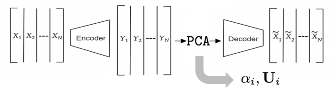
Rank reduction auto-encoder

The RRAE constructs a low dimensional linear manifold of dimension R that enables robust interpolation and generation. Several studies [28, 29] have investigated the integration of PCA in autoencoders and generative networks but focused primarily on interpretability, control and offline processes. To our knowledge we are the first in [27] to showcase its potential for screening and optimization processes requiring fast and reliable generative capabilities.

Regression

The RRAE thus allows for generative capabilities but its application for regression in a surrogate modeling approach remains to be addressed. We recall the objective being to enable the retrieval of solutions $\textbf{X}$ from designs given by sets of parameters $\mathbf {\mu }$.

The formalism of the nonlinear reduction provided by the autoencoders and described previously allows us to express $\mathbf {\mu }$ and $\textbf{X}$ using Eq. 2 and Eq. 3 respectively.

$$\begin{aligned} \tilde{\mathbf {\mu }} = \mathcal {N}^{\mathbf {\mu }}_{\mathbf {\theta }^d}(\mathcal {N}^{\mathbf {\mu }}_{\mathbf {\theta }^e}(\mathbf {\mu })) = \mathcal {N}^{\mathbf {\mu }}_{\mathbf {\theta }^d}(Y_{\mathbf {\mu }}) \end{aligned}$$

(2)

$$\begin{aligned} \tilde{\textbf{X}} = \mathcal {N}^{\textbf{X}}_{\mathbf {\theta }^d}(\mathcal {N}^{\textbf{X}}_{\mathbf {\theta }^e}(\textbf{X})) = \mathcal {N}^{\textbf{X}}_{\mathbf {\theta }^d}(Y_{\textbf{X}}) \end{aligned}$$

(3)

The application of the truncated PCA in the latent space then allows formulating $Y_{\mathbf {\mu }}$ and $Y_{\textbf{X}}$ as Eq. 4 and Eq. 5 respectively.

$$\begin{aligned} Y_{\mathbf {\mu }} = \sum _{i=1}^{R_{\mathbf {\mu }}} \alpha _i(\mathbf {\mu }) \textbf{A}_i \end{aligned}$$

(4)

$$\begin{aligned} Y_{\textbf{X}} = \sum _{i=1}^{R_{\textbf{X}}} \beta _i(\textbf{X}) \textbf{B}_i \end{aligned}$$

(5)

With $\alpha _i$ and $\textbf{A}_i$ respectively the weight coefficients and the vectors from a common reduced basis $\{ \textbf{A}_1,...,\textbf{A}_{R_{\mathbf {\mu }}} \}$ defining the parametrization of the design in the reduced space learned by the encoder $\mathcal {N}^{\mathbf {\mu }}_{\mathbf {\theta }^e}$. And $\beta _i$ and $\textbf{B}_i$ respectively the weight coefficients and the vectors from a common reduced basis $\{ \textbf{B}_1,...,\textbf{B}_{R_{\textbf{X}}} \}$ defining the parametrization of the solution in the reduced space learned by the encoder $\mathcal {N}^{\textbf{X}}_{\mathbf {\theta }^e}$. In order to express $\textbf{X}$ as $\mathbf \mu$, one must only find a mapping $f_{\alpha \text {-}\beta }$ between both sets of coefficients $\alpha _i$ and $\beta _i$. This mapping can be found using several methods and we choose in this study to learn it using a multi-layer perceptron (MLP).

The generative modeling framework can then be summarized as in Eq. 6.

$$\begin{aligned} \tilde{\textbf{X}} = \mathcal {N}^{\textbf{X}}_{\mathbf {\theta }^d}(f_{\alpha \text {-}\beta }(\mathcal {N}^{\mathbf {\mu }}_{\mathbf {\theta }^e}(\mathbf {\mu }))) \end{aligned}$$

(6)

Figure 3 allows illustrating the full range of applicability of the RRAE method as both a regressor and a generator. In a dual $\mathbf {\mu }$/$\textbf{X}$ setting, the training of the paired autoencoders as seen in Fig. 3aallows for the learning of meaningful and linearly interpolable latent representations of both the designs and their solutions. The mapping $f_{\alpha \text {-}\beta }$ between coefficients of both latent spaces then enables the regression of solutions for any given set of design parameters as shown in Fig. 3bhighlights this process showing the simultaneous generation of new designs and their associated solutions based on two known designs $\mathbf {\mu }_1$ and $\mathbf {\mu }_2$ only.

Fig. 3

Summary of the RRAE capabilities

Optimization of a vacnt-based air-filled waveguide for millimeter wave

In this section, we considered a vertically aligned carbon nanotube (VACNT)-based air-filled waveguide (AFWG) as original study case to demonstrate that

• 1. Rank-Reduction AutoEncoders (RRAE) [27], can be applied with high efficiency for the design of complex RF components. The major challenge addressed in this work consists in building a parametric model from simulated S parameters, which exhibit many localizations due to resonant frequencies. Previous works have applied alignment techniques to address these issues, in several automotive engineering applications [30,31,32,33]. In the current study, we consider a technique based on the use of the so-called RRAE [27], that has a strong potential to solve such mathematical problem with high efficiency.

• 2. this new CNT-based component can be a valuable alternative to classical technologies for millimeterwave application. By using VACNT walls instead of typical metallic walls we were able to fabricate high integrated WG and by using air as the propagation medium, the transmission losses should be reduced, showing that this design could work for future wire-less communication systems.

Background and modeling

This study extends the prior investigations presented in [3, 4], which introduced an air-filled waveguide structure utilizing vertically aligned carbon nanotube (VACNT) walls in place of conventional metallic sidewalls for E-band applications. That design employed a silicon substrate on the upper side and alumina on the lower side. The waveguide supports the dominant $TE_{10}$ mode and is excited through a transition from a grounded coplanar waveguide (GCPW) to the air-filled CNT-based waveguide. Electromagnetic confinement is achieved through input and output terminations formed by vertically aligned CNT pillars. The experimental realization of this E-band waveguide, as detailed in [3], demonstrated promising performance metrics and validated the proposed concept.

The electromagnetic behavior of the CNT walls is modeled using the Ansys HFSS solver, incorporating a frequency-dependent bulk conductivity model tailored for the CNT forest. The model captures the influence of angular frequency and CNT density, expressed in terms of the number of single-walled CNTs per unit volume ($D_\text {CNT}$), as described in Equ. 7:

$$\begin{aligned} \sigma _{\text {axial}} = \frac{8e^2 v_F}{h(v+j\omega )} D_\text {CNT} \end{aligned}$$

(7)

Here, $v_F$, v, and $D_\text {CNT}$ corresponds to fermi velocity of CNT, relaxation frequency, and density of CNT bundle, respectively. This model considers the perfect alignment of CNTs as well as their single-walled nature. The VACNT walls are 500 $\mu$m in width and 100 $\mu$m in height. We assumed a gold conductivity of $4.5 \cdot 10^7$ S/m on top and bottom and a CNT density of $10^{15}$ CNTs/$m^2$ to get a theoretical VACNT conductivity of $2.3 \cdot 10^5$ from 7. The isometric view of the device is illustrated in Fig. 4.

Fig. 4

Isometric view of the device configuration

Design and key optimization parameters

Having introduced the theoretical modeling and structure of the VACNT-based waveguide, we now focus on the key geometric parameters that influence its electromagnetic performance and the setup of our design space exploration. This work aims to develop and optimize a novel D-band AFWG structure by building upon the technological framework introduced in [3]. Unlike the previous design, where the fundamental $TE_{10}$ mode was excited via vertically aligned CNT pillars, the current approach replaces this with input/output access lines to simplify fabrication. The excitation is achieved through modified coplanar waveguide (CPW) structures, which are patterned onto a gold metallization layer deposited on the lower alumina substrate. Figure 5 displays the D-band AFWG schematic that is inspired from [3].

This application targets an operational frequency band ranging from 135 to 155 GHz. The electromagnetic response is characterized by the scattering parameters $S_{11}$ and $S_{21}$, where $S_{11}$ represents the input reflection coefficient and $S_{21}$ represents the transmission coefficient. In the following, the quantities used for training, prediction, plotting, and optimization are their dB magnitude responses, denoted as $|S_{11}|_{\textrm{dB}}$ and $|S_{21}|_{\textrm{dB}}$, with $|S_{ij}|_{\textrm{dB}} = 20\log _{10}|S_{ij}|$. In practice, an optimal design exhibits low $|S_{11}|_{\textrm{dB}}$ values while maintaining $|S_{21}|_{\textrm{dB}}$ as close to 0 dB as possible across the frequency band of interest. In this work, the design objective is to achieve $|S_{11}|_{\textrm{dB}} < -10$ dB and $|S_{21}|_{\textrm{dB}} > -5$ dB over at least 10 GHz within the 135–155 GHz target band.

Fig. 5

Schematic of the proposed waveguide. The model parameters are: WG L= 6, W= 1.4, Alumina Sub L= 10.4, Alumina Sub W= 3.8, Gold Met L = 9.4, Gold Met W= 2.8, and CNT Wallw = 0.5 (Units: mm)

To optimize the electromagnetic transition from the coplanar waveguide (CPW) to the carbon nanotube (CNT)-based air-filled waveguide, five geometric parameters p1, p2, p3, p4 and p5 were examined, as depicted in Fig. 6. These include:

• the CPW feed depth $D_{CPW}$ (p1), which defines the length of CPW that extends into the CNT cavity relatively to the waveguide wall or iris. It ranges from 0 to 1.35 mm.

• the taper center offsets $X_t$ (p2) and $Y_t$ (p3), representing horizontal and vertical displacement from a central reference aligned with the taper geometry. In this implementation they are expressed as absolute coordinates and range from 55 to 465 $\mu m$ and 1.5 to 3 mm respectively.

• the taper width $W_t$ (p4), governing the aperture through which energy is coupled into the waveguide. Its value varies between 50 and 460 $\mu m$.

• the via spacing $V_{space}$ (p5), which controls the separation between the CPW feed and adjacent via structures for electromagnetic shielding or ground continuity. It varies within the 30 to 50 $\mu m$ range.

Fig. 6

Identification of the design parameters

All the ranges of dimensions for parameters p1 to p5, satisfy fabrication constraints imposed by the technological process. These parameters were varied to study their influence on insertion loss, return loss, and overall mode-matching performance between the CPW and the CNT-based waveguide by ways of monitoring $|S_{11}|_{\textrm{dB}}$ and $|S_{21}|_{\textrm{dB}}$ curves. Together, these five variables define a compact but constrained transition-design space. The taper position and aperture width are not independent in practice, since some combinations lead to geometrically inconsistent transitions. Similarly, the CPW penetration depth and via spacing influence the coupling region while remaining bounded by fabrication and layout constraints. The resulting design space is therefore not only low-dimensional, but also correlated and partially constrained. This makes it a relevant test case for evaluating whether a surrogate model can learn feasible regions of the design space from a limited DoE, instead of relying solely on manually refined parameter sweeps.

This design of experiment (DoE) led to the creation of a database comprising 421 designs together with their respective $|S_{11}|_{\textrm{dB}}$ and $|S_{21}|_{\textrm{dB}}$ curves. Figure 7 showcases the dataset in terms of $|S_{11}|_{\textrm{dB}}$. The HFSS simulation setup used for generating this high-fidelity database is summarized here. The full-wave simulations were performed in Ansys HFSS using the driven-modal solution type. Adaptive meshing was carried out at a solution frequency of 150 GHz with a convergence criterion of $\Delta S$ = 0.02 and a maximum number of 25 adaptive passes. Since the geometry varies across the DoE samples, the final mesh size, number of completed adaptive passes, and total simulation time may vary from one design to another. The representative computational cost associated with a high-fidelity HFSS evaluation is estimated to require between 10 and 20 min.

Fig. 7

Dataset of $|S_{11}|$ responses across the 421 simulated designs

AI Surrogate model

With the dataset of waveguide designs and corresponding simulation results established, we proceed to describe the machine-learning-based surrogate modeling framework employed for rapid performance prediction and generative design.

The RRAE method described in Sect.  “Generative surrogate modeling” is particularly suited to generative design applications. Its ability to promote compact low-rank latent representations makes it suitable for limited-data settings and efficient latent-space exploration.

In the present generative engineering-design setting, the RRAE formalism is applied in a parallel/dual setting. On one hand a RRAE is tasked with learning a self-mapping from a set of design parameters $\mathbf {\mu }$ while generating a reduced latent representation $Y_{\mathbf {\mu }}$ of rank $R_{\mathbf {\mu }}$. On the other hand a RRAE is tasked with learning another self-mapping from a set of solutions $\textbf{X}$ to their reduced latent representation $Y_{\textbf{X}}$ of rank $R_{\textbf{X}}$.

It should be mentioned that this paired autoencoder setting is formulated to be applicable in the widest range of applications but is not always a necessity. As stated in Sect. “Generative surrogate modeling”, its use targets applications involving dimensionality reduction or highly-correlated and non-parametric data. Although the present input space contains only five parameters, these parameters are geometrically correlated and subject to feasibility constraints. The design-side RRAE is therefore retained in this study to keep the formulation consistent with the general dual-RRAE framework and to demonstrate how the method can be applied when the design representation is correlated, higher-dimensional, or non-parametric.

By design and as explained in Sect. “Generative surrogate modeling” this defined formalism leads to the learning of latent spaces whose representative coefficients can be linearly interpolated. Therefore, new designs $\mathbf {\mu }_n$ or new solutions $\textbf{X}_n$ can simply be obtained by interpolating new coefficients $\alpha ^n_i$ or $\beta ^n_i$ from sets of representative coefficients of any known designs or solutions.

In our case the previously defined $\mathbf {\mu }$ and $\textbf{X}$ refer to sets of design parameters [$D_{CPW}$,$X_t$, $Y_t$,$W_t$,$V_{space}$] and sets of solutions [$|S_{11}|_{\textrm{dB}}$,$|S_{21}|_{\textrm{dB}}$] respectively. In practice, the input $\mathbf {\mu }$ is a vector containing the standardized values of the 5 design parameters. As for the output $\textbf{X}$, it is a matrix of dimension (2,$n_f$) where the 2 rows contain the normalized $|S_{11}|_{\textrm{dB}}$ and $|S_{21}|_{\textrm{dB}}$ curves respectively and where $n_f$ is the number of points sampled for each curve in HFSS. In this work a sampling frequency of 200 MHz was chosen and therefore both $|S_{11}|_{\textrm{dB}}$ and $|S_{21}|_{\textrm{dB}}$ contain 251 points within our 110–160 GHz range. In practice, the two normalized S-parameter channels are augmented with Fourier positional features along the frequency axis. Ten sine–cosine frequency pairs are concatenated to the original $|S_{11}|_{\textrm{dB}}$ and $|S_{21}|_{\textrm{dB}}$ channels, resulting in $2+2\times 10=22$ input channels.

In this application the objective is to be able to retrieve the associated solutions to any given parameter choice. According to Eq. (2) and Eq. (3), one only needs to find the correlation $f_{\alpha \text {-}\beta }$ that relates the coefficients $\alpha$ characterizing each design in its latent space to the coefficients $\beta$ characterizing their associated solution in the latent space of the solutions.

There are several approaches to establish the correlation between the reduced design coefficients $\alpha$ and the reduced response coefficients $\beta$. In this work, this correlation is learned using a multi-layer perceptron (MLP), denoted $f_{\alpha \rightarrow \beta }$. The complete surrogate is therefore composed of three main elements: a design RRAE that maps the design parameters to reduced coefficients $\alpha$, a response RRAE that maps the S-parameter magnitude curves to reduced coefficients $\beta$, and a coefficient mapper that learns the relation between both reduced spaces.

Due to the structure of the data, the design RRAE is implemented using fully connected encoder and decoder networks, whereas the response RRAE uses one-dimensional convolutional encoder and decoder networks operating along the frequency axis. The convolutional blocks use a kernel size of 3, stride 1, replicate padding, batch normalization, and LeakyReLU activation, except for the final output layer. The coefficient mapper is also fully connected and maps the reduced design coefficients $\alpha$ to the reduced response coefficients $\beta$.

The rank-reduction stage is inserted between the encoder and decoder of each autoencoder. It is implemented as a truncated SVD/PCA-like projection applied in the latent space. The design latent space has dimension 256 and is reduced to rank $R_{\mu }=6$, while the response latent space has dimension 128 and is reduced to rank $R_{X}=14$. In both cases, the decoder reconstructs the data from the projected low-rank latent representation rather than from the unconstrained encoder output. The complete architecture is summarized in Table 1.

Table 1 Summary of the RRAE and direct regression baseline architectures

The training and use of this architecture are decomposed into three steps. Algorithm 1 first describes the training of a single RRAE block, which is common to both the design and response autoencoders. Algorithm 2 then describes the complete training procedure of the coupled surrogate, including the extraction of the reduced coefficients and the learning of $f_{\alpha \rightarrow \beta }$. Finally, Algorithm 3 describes how the trained pipeline is used either for prediction from a prescribed design or for generation from interpolated design coefficients.

Algorithm 1

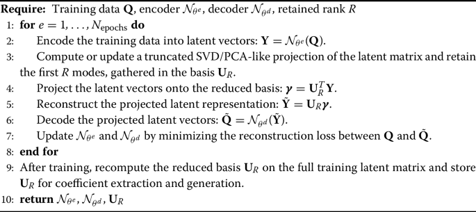
Training of a single RRAE model

Algorithm 2

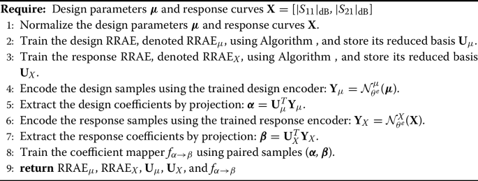
Training of the complete RRAE surrogate pipeline

Algorithm 3

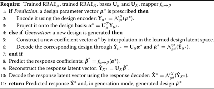
Prediction and generation using the trained RRAE surrogate

The database obtained from the DoE was divided into training and test sets using a 70/30 split. The training set was used to train the design and response RRAEs, as well as the coefficient mapper $f_{\alpha \rightarrow \beta }$. The test set was reserved for assessing the prediction accuracy of the complete surrogate model. Both RRAEs were trained with the same settings: a learning rate of $10^{-4}$, the Adam optimizer, a mean-square error reconstruction loss, and a batch size of 40. A cosine annealing scheduler with warm restarts was used for the learning rate.

To ensure a controlled evaluation, we compare the RRAE surrogate with a direct encoder-decoder regression baseline. This baseline is built from the same design encoder $\mathcal {N}^{\mathbf {\mu }}_{\mathbf {\theta }^e}$ and response decoder $\mathcal {N}^{\textbf{X}}_{\mathbf {\theta }^d}$ as the RRAE surrogate, as illustrated in Fig. 8. The difference is that the direct baseline removes the truncated SVD/PCA rank-reduction blocks and directly maps the design parameters to the response curves. This construction provides a fair comparison in terms of pointwise regression capacity while isolating the contribution of the structured low-rank latent representation and interpolation mechanism.

Both models are trained using the same database, train/test split, normalization procedure, optimizer, loss function, learning rate schedule, and batch size. No exhaustive hyperparameter optimization was performed, since the purpose of the comparison is not to identify the best possible regressor for this dataset, but to compare two surrogate-assisted screening workflows under the same learning conditions. More complex architectures, such as attention-based models or adversarial generative models, could also be considered for response prediction or inverse design. However, introducing such models would change both the network capacity and the training assumptions, making it harder to isolate the effect of the RRAE rank-reduction stage. The direct encoder–decoder baseline is therefore intended to represent a usable screening surrogate rather than an extensively optimized digital-twin model. Its performance in comparison to the RRAE is assessed hereafter.

Fig. 8

Direct encoder–decoder regression baseline based on the RRAE backbone, without the rank-reduction stage

Results and discussion

After training the surrogate models, we evaluate their prediction accuracy and generative capabilities, followed by a discussion of key findings from the design optimization.

Regression performance and full-band reconstruction fidelity

Before evaluating the use of the surrogate models for design exploration, we first assess their ability to reproduce the electromagnetic responses obtained with HFSS over the full simulated frequency range. This step is important because the objective is not only to identify designs satisfying a specific requirement, but also to verify that the surrogate captures the overall behavior of both well-performing and poorly-performing designs across the investigated design space.

Prediction quality is evaluated using full-band reconstruction metrics computed directly on the denormalized $|S_{11}|_{\textrm{dB}}$ and $|S_{21}|_{\textrm{dB}}$ curves. For each test sample, the mean absolute error (MAE) is first computed over the full simulated frequency range. The resulting sample-wise error distribution is then summarized using the median and the 90th percentile, denoted Q90. The median MAE characterizes the typical reconstruction error, while Q90 indicates the error level below which 90% of the test samples fall. Reporting Q90 therefore provides information on the upper tail of the error distribution and helps assess reconstruction robustness without relying only on the worst-case sample, which may be dominated by isolated outliers.

Since MAE is expressed in dB, an additional dimensionless metric is included to facilitate interpretation beyond an RF-specific scale. The standardized MAE (sMAE) is obtained by normalizing the sample-wise MAE by the standard deviation of the corresponding HFSS response over the test set. It therefore expresses the reconstruction error relative to the natural variability of the simulated responses. For example, an sMAE of 0.15 indicates that the typical reconstruction error corresponds to approximately 15% of the standard deviation of the HFSS responses in the test set.

In addition to pointwise error metrics, the full-curve Pearson correlation is computed between each predicted response and its corresponding HFSS response. This metric measures the similarity of the frequency-dependent trends independently of the absolute error magnitude. It is therefore useful for assessing whether the surrogate captures the overall shape of the response, including slopes, resonant variations, and broadband tendencies. Together, the MAE, sMAE and correlation metrics provide complementary information on absolute reconstruction error, scale-independent error, and curve-shape preservation.

Table 2 Full-band reconstruction performance on the test set

The results in Table 2 show that both surrogate models provide comparable full-band reconstruction accuracy. For $|S_{11}|_{\textrm{dB}}$, the RRAE reaches a median MAE of 0.41 dB and a 90th-percentile MAE below 1 dB, indicating that the return-loss response is accurately reconstructed for most test samples. The direct baseline exhibits a very similar behavior, with a median MAE of 0.42 dB and a 90th-percentile MAE of 1.00 dB. These results suggest that both models are able to reproduce the main $|S_{11}|_{\textrm{dB}}$ response over the investigated design space.

The reconstruction of $|S_{21}|_{\textrm{dB}}$ is more challenging in terms of absolute dB error, with median MAE values of 3.25 dB for the RRAE and 3.37 dB for the the direct encoder-decoder baseline. However, the median full-curve correlations remain high for both models, around 95%, indicating that the global frequency-dependent trends of the transmission response are preserved despite larger local amplitude deviations. The standardized MAE values also remain moderate, with typical errors corresponding to approximately 15% of the test-set variability for $|S_{11}|_{\textrm{dB}}$ and 20% for $|S_{21}|_{\textrm{dB}}$. This indicates that the prediction errors remain limited relative to the natural variability of the simulated responses.

The gap between the median and Q90 errors remains moderate for $|S_{11}|_{\textrm{dB}}$, with a Q90 MAE below 1 dB for both models. This indicates that accurate reconstruction is not limited to a few favorable test samples but is maintained for most of the test set. For $|S_{21}|_{\textrm{dB}}$, larger dB errors are observed, with Q90 values around 5 dB. However, the median correlations remain close to 95%, suggesting that the global frequency-dependent transmission trends are preserved even when local amplitude deviations are larger. Representative reconstructions are shown in Fig. 9, comparing HFSS, RRAE and direct baseline predictions on test-set examples.

Fig. 9

Comparison of RRAE, direct encoder-decoder baseline, and HFSS predictions of S-parameter magnitudes for a given VACNT-AFWG design

Overall, this analysis indicates that the RRAE and encoder-decoder baseline exhibit similar reconstruction fidelity when considered purely as regression models. Therefore, the contribution of the RRAE should not be interpreted as a major improvement in pointwise prediction accuracy. Rather, the importance of the RRAE lies in the structure of its latent representation: while maintaining regression accuracy comparable to that of the direct baseline, it provides an interpolable low-rank design space that can be exploited for constraint-preserving candidate generation and efficient design exploration, as discussed in the following subsection.

AI-based design optimization

The previous subsection showed that the RRAE and the direct encoder–decoder baseline provide comparable full-band reconstruction accuracy when considered purely as regression models. The distinction between the two approaches therefore lies primarily in how they can be used during design-space exploration. For a single forward prediction, both methods provide millisecond-scale inference: on the surrogate-modeling hardware used in this study (CPU: AMD Ryzen 7 6800 H, GPU: RTX 3060 M, VRAM: 6GB, RAM: 16GB), the prediction of the full $|S_{11}|_{\textrm{dB}}$ and $|S_{21}|_{\textrm{dB}}$ responses for one design takes approximately 4.9 ms with the direct baseline and 5.9 ms with the RRAE. In comparison, one HFSS simulation requires approximately 10–20 min on the simulation workstation (CPU: Intel Core i9-13900 H, GPU: RTX 4070 M, VRAM: 8GB, RAM: 64GB), depending on the mesh and convergence conditions.

However, the objective of the proposed framework is not only fast prediction of isolated parameter sets. The purpose is to support design-space exploration by generating and evaluating candidate designs. In this respect, the two approaches differ fundamentally. The direct encoder–decoder baseline requires externally provided design parameters and therefore depends on an explicit sampling strategy in the original parameter space. By contrast, the RRAE learns a structured latent representation of the design data, allowing new candidate designs to be generated by interpolation within the learned low-rank latent space before response prediction.

This distinction is important for optimization workflows. Even in the present five-parameter case, the admissible design space is not a simple Cartesian product of independent variables, because geometric correlations determine whether a sampled parameter set corresponds to a feasible transition. As the number of variables or constraints increases, exhaustive parameter sweeps and sensitivity-driven refinements rapidly become costly. The RRAE does not remove the need for final HFSS validation, but it provides a mechanism for proposing candidate designs from within the learned data manifold, thereby reducing the reliance on manually designed sampling rules during exploration.

The optimization strategy chosen in this study exploits the ability of both methods to quickly review possible designs. It consists in rapidly exploring a range of possible designs and evaluating their associated solutions with the objective of satisfying set requirements. In this work, the search for optimal designs is formulated as the minimization of a goal function G given in Eq. (8). As previously defined, the objective is to minimize the amplitude of $|S_{11}|_{\textrm{dB}}$ while ensuring $|S_{21}|_{\textrm{dB}}$ remains as close to 0 as possible on the condition that $|S_{11}|_{\textrm{dB}}$ is below the threshold of -10 dB for at least 10 GHz in the 135 to 155 GHz range. Since candidate designs are required to satisfy the $|S_{21}|_{\textrm{dB}}>-5$ dB transmission condition, the scalar objective $G$ is formulated using $|S_{11}|_{\textrm{dB}}$ among candidates satisfying this constraint.

$$\begin{aligned} G = \int _{f_1}^{f_2} |S_{11}|_{\textrm{dB}}\, df \end{aligned}$$

(8)

where $f_1$ and $f_2$ denote the lower and upper frequencies of the interval over which $|S_{11}|_{\textrm{dB}}<-10$ dB.

To start with, and to gauge the difficulty of satisfying this optimization criterion, we review all of the 421 designs simulated with HFSS in order to identify potentially matching candidates already present in our dataset.

Out of the 421 designs, only 1 was found to meet the target requirements. Not only does it highlight the challenge of optimizing our chosen design but it also indicates that the database used for the learning of both the direct baseline and the RRAE methods is scarce in examples meaningful for our case. The robustness and generalization capacity of both methods will therefore be put to test in order to come up with relevant designs and accurate solutions.

Based on the set criterion, a design search is set up for both the direct encoder–decoder baseline and the RRAE method. This design search requires a thorough exploration of the design space along with the associated solutions. As the encoder-decoder baseline and RRAE are fundamentally different in terms of generation we hereby define their respective exploration strategies.

As stated previously, the direct baseline does not involve any generative component. Navigating the design space hence relies on the prior knowledge of an explicit parametrization of the designs. In our present case, this parametrization is made using the 5 parameters p1 to p5 defined in Sect. “Optimization of a vacnt-based air-filled waveguide for millimeter wave” and shown in Fig. 11. The range of these parameters is set and possible correlations between them are known. To ensure the geometrical consistency of the design we know for instance that p3 and p4 are interdependent and that consequently some combinations of values will lead to erroneous geometries. To explore the design space using the direct baseline we shall then uniformly sample possible parameter combinations. In order to compare both methods on the same basis we ignore here parameter correlations during the sampling to better represent the challenges of optimizing complex engineering designs. A total of 9,765,625 designs are hence assessed using the baseline method by sampling unique 5-parameter combinations.

The generation process of the RRAE, explained in Sect. “Generative surrogate modeling” and summarized in Fig. 3c

The summary of the results of the design search for both surrogate-assisted workflows is given in Table 3. The design search using the direct baseline and RRAE approaches took around 3h07min and 1h50min, respectively, corresponding to 872 designs reviewed per second for the direct baseline and 1102 designs reviewed per second for the RRAE. These time frames highlight the potential of surrogate-based workflows for rapid design screening. For comparison, only on the order of 5–20 designs could have been assessed using HFSS in the same time range, assuming 10–20 min per full-wave simulation.

To better quantify the computational cost at the workflow level, the upfront cost of generating the initial database should also be considered. The 421 HFSS simulations used for training represent an equivalent serial simulation cost of approximately 70–140 h. Once this initial cost has been paid, the trained surrogates can screen candidates at millisecond-scale rates. At the measured RRAE screening rate, the same equivalent time required to generate the initial HFSS database would allow approximately $2.8\times 10^8$ to $5.5\times 10^8$ candidate designs to be evaluated. This comparison does not imply that HFSS validation is replaced. Rather, it illustrates how a limited high-fidelity simulation budget can be converted into a large-scale design exploration capability.

Table 3 Computational cost and outcome of the surrogate-assisted design searches

The search led to the identification of 807,539 potential valid designs using the RRAE and 548 using the direct baseline. Since both surrogate models showed comparable full-band reconstruction accuracy in the previous subsection, this difference should not be attributed primarily to pointwise prediction accuracy. Rather, it reflects the different exploration mechanisms. With the direct baseline, exploration relies on explicit parameter-space sampling, whose effectiveness depends on the sampling resolution and on the manual handling of geometric constraints. By contrast, the RRAE generates new candidates by interpolation in the learned low-rank latent space, allowing the search to focus on regions consistent with the design manifold learned from the initial HFSS database.

As the potential designs identified using both methods likely contain very closely related designs we apply once again the design uniqueness criterion requiring parameter sets to have a relative difference of at least 10%. 8 unique designs are hence identified using the RRAE and 10 with the direct baseline. Here, the more exhaustive search only permitted by the knowledge of the design parametrization, may have allowed for the retrieval of 2 more unique designs with the encoder-decoder baseline. Their consistency however still needs to be verified. In addition, a less random approach for data generation during the DoE would have likely avoided this difference.

These potential designs found using both methods ought to be verified using HFSS in order to assess both (i) the consistency of the design with regard to the geometrical constraints and (ii) the validity of the high-fidelity solution with regard to the optimization criterion.

Among the 8 designs found using the RRAE framework all were found to be geometrically consistent and 5 of them were confirmed to meet the objective which leaves 3 under-performing design due to inaccuracies in the prediction of the model. The $|S_{11}|_{\textrm{dB}}$ and $|S_{21}|_{\textrm{dB}}$ curves of each of the 5 candidates retrieved using the RRAE method and validated using HFSS appear in Fig. 10.

Fig. 10

Valid unique RRAE solutions

As for the 10 designs found with the direct encoder–decoder approach, 5 were found to be geometrically inconsistent and the remaining 5 did not satisfy the 10 GHz bandwidth condition. These geometrical inconsistencies could have been avoided by explicitly enforcing the known correlations between design parameters during sampling; however, this highlights a limitation of direct parameter-space exploration when feasibility constraints must be handled manually.

In comparison, all RRAE candidates retained for HFSS validation were geometrically consistent. This suggests that interpolation within the learned low-rank design manifold preserved the main parameter correlations present in the DoE, without requiring them to be explicitly imposed during generation.

Regarding the remaining 5 under-performing designs obtained with the direct encoder–decoder baseline, it is unlikely that all of them are due to the model inaccuracy as both of the methods show comparable levels of precision. Another more likely reason is the limited ability of the direct encoder-decoder baseline to generalize to these unseen candidate designs. Indeed, inverse engineering design issues tackled in literature and exploiting this approach often rely on a vast amount of data to train models in order to ensure generalization. For instance, the authors in [14] use between 60k and 180k sets of data to optimize the design of integrated circuits. In comparison, our 421 sets can appear very limiting but much more realistic and scalable in terms of requirements in a practical industrial setting. The frugality of the RRAE and its ability to capture relevant information to generalize even based on limited data makes it particularly relevant in this context.

Finally, a comparison is made in Fig. 11 between the solutions of the valid design from the DoE and the solutions of the best design provided by the RRAE generative model according to our optimization criterion. Table 4 showcases the parameters of the unique designs found using AI and the valid one from the DoE as well as the value of the optimization metric and the obtained bandwidth.

Fig. 11

Best of DoE vs Best of RRAE solutions

Table 4 Comparison of valid DoE and RRAE-generated designs with associated optimization metric G ($\downarrow$) and bandwidth $\Delta f$

Table 4 illustrates the varied range of different designs that can be obtained using the RRAE approach. The generation through latent space exploration enables a very fast and thorough assessment of design validity based on the overall knowledge of possible design parameterizations and sets of solutions gathered from a set of real representative examples. Despite the dataset including only 1 valid design, the RRAE approach was able to generalize beyond known solutions by not only providing variety in terms of designs but improvements in terms of performance. Indeed, most of the unique designs retrieved using the RRAE appear to outperform the DoE design, highlighting its potential for design optimization. The designs retrieved can then be used as a basis for further refinement using high-fidelity tools such as HFSS, which is particularly advantageous in terms of time efficiency, especially when handling a large number of correlated parameters or operating in non-parametric settings.

Conclusions

This work presented a new application of the rank-reduction autoencoder (RRAE) framework for the design and optimization of RF and microwave components. The RRAE is proposed here as a generative surrogate modeling approach reconciling two common limitations of AI-based engineering optimization frameworks: frugality and explorability. By embedding a truncated PCA stage within an autoencoder architecture, the RRAE enables robust interpolation and constraint-preserving generative sampling from limited data.

The optimization of a VACNT-based air-filled waveguide was adopted here as a case study, targeting D-band operation. Based on 421 simulations obtained using HFSS, the RRAE allowed the retrieval of 5 unique optimized designs with operational bandwidths between 135 and 155 GHz. A comparison is made with a direct encoder-decoder regression baseline without the rank-reduction stage. Although this baseline achieved comparable full-band reconstruction accuracy, it did not produce any HFSS-confirmed valid design in the proposed screening workflow.

These results demonstrate that the RRAE can substantially reduce computational costs by leveraging its efficient generative capabilities, enabling fast and reliable convergence towards optimal designs. In doing so, it minimizes the need for extensive parametric studies, hence offering a scalable strategy for AI-driven optimization of emerging low-loss waveguide technologies. Beyond the present case study, the framework provides a generalizable approach that can be extended to other RF components (such as cavity, filter and antennas) where data efficiency and design explorability are critical.

References

Huang T, Yang W, Wu J, Ma J, Zhang X, Zhang D. A survey on green 6g network: architecture and technologies. IEEE Access. 2019;7:175758–68. https://doi.org/10.1109/ACCESS.2019.2957648.
Bertrand M, Pistono E, Acri G, Kaddour D, Podevin F, Puyal V, Wipf ST, Wipf C, Wietstruck M, Kaynak M, Ferrari P. Substrate integrated waveguides for mm-wave functionalized silicon interposer. In: 2018 IEEE/MTT-S International Microwave Symposium - IMS, 2018; pp. 875–878. https://doi.org/10.1109/MWSYM.2018.8439287
de Saxcé JM, Siah CF, Wei TC, Passerieux D, Bila S, Podevin F, et al. E-band vertically aligned carbon nanotubes-based air-filled waveguide. IEEE Microw Wireless Technol Lett. 2023;33(4):395–8. https://doi.org/10.1109/LMWT.2022.3227946.
Kumar A, Kumar A, Jaing R, Baillargeat D, Bila S, Coquet P, Tay BK. Vertically aligned carbon nanotubes-based passive devices for mm-waves applications. In: 2024 IEEE Asia-Pacific Microwave Conference (APMC), 2024; pp. 163–165. https://doi.org/10.1109/APMC60911.2024.10867696
Kiziltas G, Psychoudakis D, Volakis JL, Kikuchi N. Topology design optimization of dielectric substrates for bandwidth improvement of a patch antenna. IEEE Trans Antennas Propag. 2003;51(10):2732–43. https://doi.org/10.1109/TAP.2003.817539.
Jiang H, Chen J, Tang K, Yan H, Hao R. Exploring high-performance slow light grating waveguides by means of deep learning. IEEE Photonics Technol Lett. 2022;34(20):1112–5. https://doi.org/10.1109/LPT.2022.3203475.
Hu X, Buris NE. A deep learning framework for solving rectangular waveguide problems. In: 2020 IEEE Asia-Pacific Microwave Conference (APMC), 2020; pp. 409–411. https://doi.org/10.1109/APMC47863.2020.9331654
Lin C-C, Na A, Wu Y-K, Wang L, Na N. Optimization of grating coupler over single-mode silicon-on-insulator waveguide to reach \({<}\) 1 db loss through deep-learning-based inverse design. Photonics. 2024. https://doi.org/10.3390/photonics11030267.
Du Z, Ding X, Chen H, Liu C, Zhang W, Luo J, et al. Optimal design of topological waveguides by machine learning. Front Mater. 2022. https://doi.org/10.3389/fmats.2022.1075073.
Xu K, Wang J, Cai J, Ma X, Lv Q, Chen S, et al. Flexible inverse design of microwave filter customized on demand with wavelet transform deep learning. Trans Comp-Aided Des Integ Cir Sys. 2025;44(3):806–17. https://doi.org/10.1109/TCAD.2024.3451329.
Volume 2: Snapshot-Based Methods and Algorithms. De Gruyter, Berlin, Boston 2021. https://doi.org/10.1515/9783110671490.
Chinesta F, Leygue A, Bordeu F, Aguado JV, Cueto E, Gonzalez D, et al. Pgd-based computational vademecum for efficient design, optimization and control. Archiv Comput Methods Eng. 2013. https://doi.org/10.1007/s11831-013-9080-x.
Kazemzadeh-Parsi M-J, Pasquale A, Di Lorenzo D, Champaney V, Ammar A, Chinesta F. Nurbs-based shape parametrization enabling pgd-based space separability: Methodology and application. Finite Elem Anal Des. 2023;227:104022. https://doi.org/10.1016/j.finel.2023.104022.
Karahan EA, Liu Z, Gupta A, Shao Z, Zhou J, Khankhoje U, et al. Deep-learning enabled generalized inverse design of multi-port radio-frequency and sub-terahertz passives and integrated circuits. Nat Commun. 2024;15:10734. https://doi.org/10.1038/s41467-024-54178-1.
Zhou Z, Wei Z, Ren J, Yin Y, Pedersen GF, Shen M. Two-order deep learning for generalized synthesis of radiation patterns for antenna arrays. IEEE Trans Artif Intell. 2023;4(5):1359–68. https://doi.org/10.1109/TAI.2022.319250.
Pan Y-Q, Wang R, Wang B-Z. Physics-informed neural networks with embedded analytical models: Inverse design of multilayer dielectric-loaded rectangular waveguide devices. IEEE Trans Microw Theory Techn. 2024;72(7):3993–4005. https://doi.org/10.1109/TMTT.2023.3343028.
Lin C-Y, Tseng T-L, Tsai T-H. A digital twin framework with meta- and transfer learning for scalable multi-machine modeling and optimization in semiconductor manufacturing. IEEE Access. 2025;13:84380–98. https://doi.org/10.1109/ACCESS.2025.3568002.
Yang G, Xiao Q, Zhang Z, Yu Z, Wang X, Lu Q. Exploring AI in metasurface structures with forward and inverse design. iScience. 2025;28(3):111995. https://doi.org/10.1016/j.isci.2025.111995.
Wang Y, Shimada K, Farimani AB. Airfoil GAN: encoding and synthesizing airfoils for aerodynamic shape optimization. J Comput Design Eng. 2023;10(4):1350–62. https://doi.org/10.1093/jcde/qwad046.
Baek SJ, Lee M. Recent advances in the inverse design of silicon photonic devices and related platforms using deep generative models. PeerJ Comput Sci. 2025;11:2895.
Ansys Inc.: Ansys HFSS | 3D High Frequency Simulation Software. https://www.ansys.com/products/electronics/ansys-hfss. Accessed 28 Aug 2025.
Wikström G, Peisa J, Rugeland P, Johansson N, Parkvall, S. Challenges and technologies for 6g. In: 2020 2nd 6G Wireless Summit (6G SUMMIT), 2020;pp. 1–5. https://doi.org/10.1109/6GSUMMIT49458.2020.9083880
Chinesta F, Cueto E, Champaney V, Ghnatios C, Ammar A, Hascoet N, Gonzalez D, Alfaro I, Lorenzo DD, Pasquale A, Baillargeat D. A gentle introduction to data, learning, and model order reduction. Springer Nature 2025. https://doi.org/10.1007/978-3-031-87572-4
Goodfellow I, Bengio Y, Courville A. Deep Learning. MITPress, Cambridge, USA 2016. https://mitpress.mit.edu/9780262035613/deep-learning/3
Schmidhuber J. Deep learning in neural networks: an overview. Neural Netw. 2015;61:85–117. https://doi.org/10.1016/j.neunet.2014.09.003.
Hinton GE, Zemel RS. Autoencoders, minimum description length and helmholtz free energy. Adv Neural Inf Process Syst. 1993;6
Mounayer J, Rodriguez S, Ghnatios C, Farhat C, Chinesta F. Rank reduction autoencoders – enhancing interpolation on nonlinear manifolds 2024. https://doi.org/10.48550/arXiv.2405.13980
Härkönen E, Hertzmann A, Lehtinen J, Paris S. Ganspace: discovering interpretable gan controls. In: Proceedings of the 34th International Conference on Neural Information Processing Systems. NIPS ’20. Curran Associates Inc., Red Hook, NY, USA 2020. https://doi.org/10.5555/3495724.3496549
Pham C-H, Ladjal S, Newson A. Pca-ae: Principal component analysis autoencoder for organising the latent space of generative networks. J Math Imaging Vis. 2022;64(5):569–85. https://doi.org/10.1007/s10851-022-01077-z.
Schmid A, Pasquale A, Ellersdorfer C, Raffler M, Champaney V, Ziane M, et al. Mechanical characterization of li-ion cells and the calibration of numerical models using proper generalized decomposition. In: Proceedings of the ASME 2023 International Mechanical Engineering Congress and Exposition IMECE2023. 2023.
Champaney V, Pasquale A, Ammar A, Chinesta F. Parametric curves metamodelling based on data clustering, data alignment, pod-based modes extraction and pgd-based nonlinear regressions. Front Mater. 2022;9:904707. https://doi.org/10.3389/fmats.2022.904707.
Pasquale A, Champaney V, Kim Y, Hascoët N, Ammar A, Chinesta F. A parametric metamodel of the vehicle frontal structure accounting for material properties and strain-rate effect: application to full frontal rigid barrier crash test. Heliyon. 2022;8:12397. https://doi.org/10.1016/j.heliyon.2022.e12397.
Schmid A, Pasquale A, Ellersdorfer C, Champaney V, Raffler M, Guévelou S, et al. Pgd based meta modelling of a lithium-ion battery for real time prediction. Front Mater. 2023. https://doi.org/10.3389/fmats.2023.1245347.
Acknowledgements
This work is supported by the National Research Foundation, Singapore, and Infocomm Media Development Authority under its Future Communications Research & Development Programme (FCP-CNRS-RG-2022-022, REQ0396559). This research is supported by the National Research Foundation, Prime Minister’s Office, Singapore under its Campus for Research Excellence and Technological Enterprise (CREATE) programme
Author information
Authors and Affiliations
Contributions
A.K. conceived the study, designed the RF waveguide and performed electromagnetic simulations, analyzed the results, and wrote the main manuscript. C.M. developed the AI-based methodology, contributed to optimization and data analysis, and assisted in writing and revising the manuscript. M.J. contributed to AI model development and optimization analysis. C.F. contributed to conceptual development, provided scientific supervision, and critically revised the manuscript. D.B. supervised the project, contributed to conceptual guidance, and revised and finalized the manuscript. All authors reviewed, approved the final version of the manuscript, and agree to be accountable for all aspects of the work.
Corresponding author
Ethics declarations
Competing interests
The authors declare no competing interests.
Additional information
Publisher's Note
Springer Nature remains neutral with regard to jurisdictional claims in published maps and institutional affiliations.
Rights and permissions
Open Access This article is licensed under a Creative Commons Attribution-NonCommercial-NoDerivatives 4.0 International License, which permits any non-commercial use, sharing, distribution and reproduction in any medium or format, as long as you give appropriate credit to the original author(s) and the source, provide a link to the Creative Commons licence, and indicate if you modified the licensed material. You do not have permission under this licence to share adapted material derived from this article or parts of it. The images or other third party material in this article are included in the article's Creative Commons licence, unless indicated otherwise in a credit line to the material. If material is not included in the article's Creative Commons licence and your intended use is not permitted by statutory regulation or exceeds the permitted use, you will need to obtain permission directly from the copyright holder. To view a copy of this licence, visit http://creativecommons.org/licenses/by-nc-nd/4.0/.
About this article
Cite this article
Kumar, A., Mailhé, C., Mounayer, J. et al. Generative surrogate modelling for the efficient design optimization of an RF component. Adv. Model. and Simul. in Eng. Sci. 13, 21 (2026). https://doi.org/10.1186/s40323-026-00340-x
Received:
Accepted:
Published:
Version of record:
DOI: https://doi.org/10.1186/s40323-026-00340-x